Introduction to Graphs
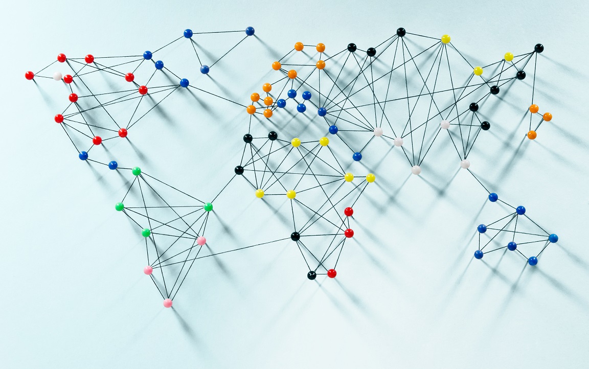
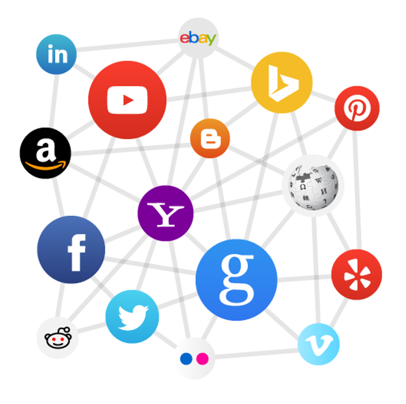
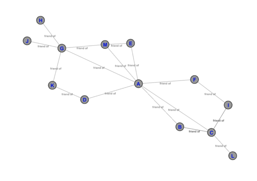
A graph is a data structure used in computer science that can be used to display different real-life problems and show features of large-scale data [1]. For example, flight connections can be displayed as a graph, where the connections are flights between 2 destinations [1]. Facebook social networks can be displayed as a graph where the connection is a friend relationship (view Figure 22). The internet is a very vast, virtual graph, where each webpage is a point, and hyperlinks denote connections between two webpages [2]. To clarify, if there is a link from a YouTube video to an Amazon link, there would be a connection between YouTube and Amazon.
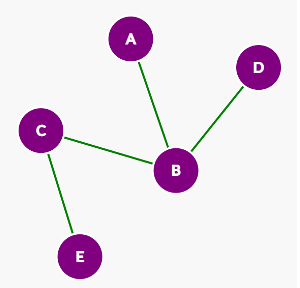
Before we dive into some well-known graph algorithms, let’s first formally define a graph. A graph is formed by a set of vertices and a set of edges. An edge denotes a connection between two vertices [3]. Edges can connect to any vertex in any way possible [4]. Note that both V1 and E1 are sets, meaning that it is a collection of elements that are unordered and unique. In the image below, the edges are represented by the green lines, and the vertices are purple circles.
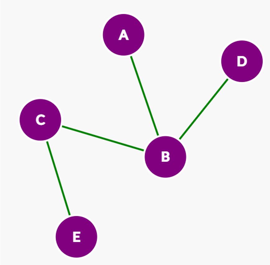
G1 = (V1, E1)
V1 = A, B, C, D, E
E1 = (A, B), (B, C), (B, D), (E, C)
Graph Terminology
Adjacency
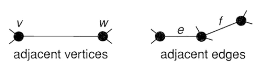
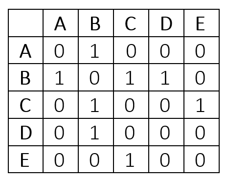
Two vertices v and w are considered adjacent if there is an edge that connects v and w [5]. Similarly, two edges e and f are considered adjacent if they share a vertex in common [5].
This relation becomes particularly useful when representing a graph as an adjacency matrix. An adjacency matrix consists of a table that is |V| x |V|, where |V| is the number of vertices in the graph. If the cell in the matrix is a 1, then that means that the edge between the two vertices exists. Likewise, if the cell is a 0, then the edge does not exist in the graph.
Subgraph
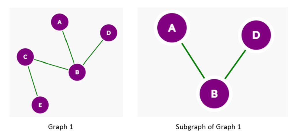
A subgraph S1 is essentially a snippet of a larger graph G1 such that the S1 is a subset of G1 and all of the edges of G1 is also an edge of G2 [3]. A subset means that every element of S1 would exist in G1. For example, the Crayola marker pack of 8 colors is a subset of the Crayola marker park of 48. Every color in the pack of 8 markets exists in the pack of 48 markers. To put this in a more visual perspective, view the example figure below.
Directed vs Undirected
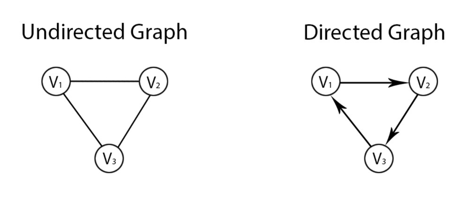
In the prior examples above, the graphs had undirected edges, which means that the between any two vertices goes in both directions [6]. A directed edge from A to B would mean that the path only exists from A to B, and typically, it is denoted by using an arrow to denote the unidirectional connection. The order of the vertices in the each edge pair matters [4]. In short, the edge (A, B) would not be equivalent to (B, A).
The Facebook social network in Figure 22, represents an undirected graph because Facebook friend request requires both users to be friends [4]. On Facebook, there is no way to be friends with someone that is not friends with you [4]. The relation is bidirectional and mutual. On Twitter, users can “follow” one other, but do not have to both “follow” one another. This means that you are able to follow Bill Gates, even though Bill Gates does not follow you back [4]. This would be best represented as a directed graph where the arrow begins at A and points to B.
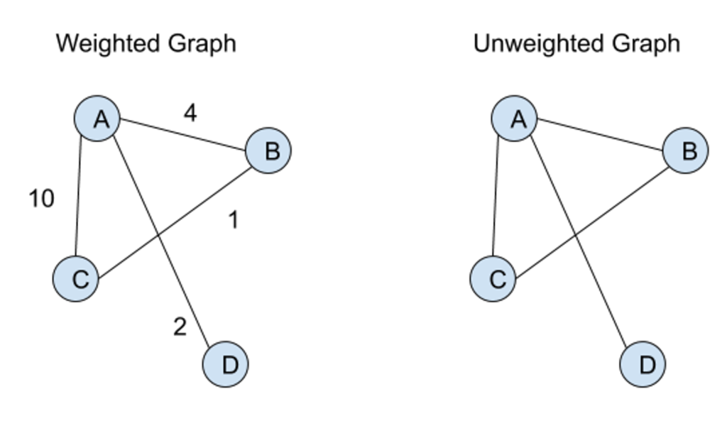
Weighted vs Unweighted
Furthermore, another specification that can be made is whether the edges consist of weighted edges. A graph with all weighted edges is denoted as a weighted graph, which are particularly useful when the problem at hand involves a quantified relationship. A weighted graph is used to represent the distance between all of the vertices on the graph or can be used to represent other quantitative data between any two vertices.
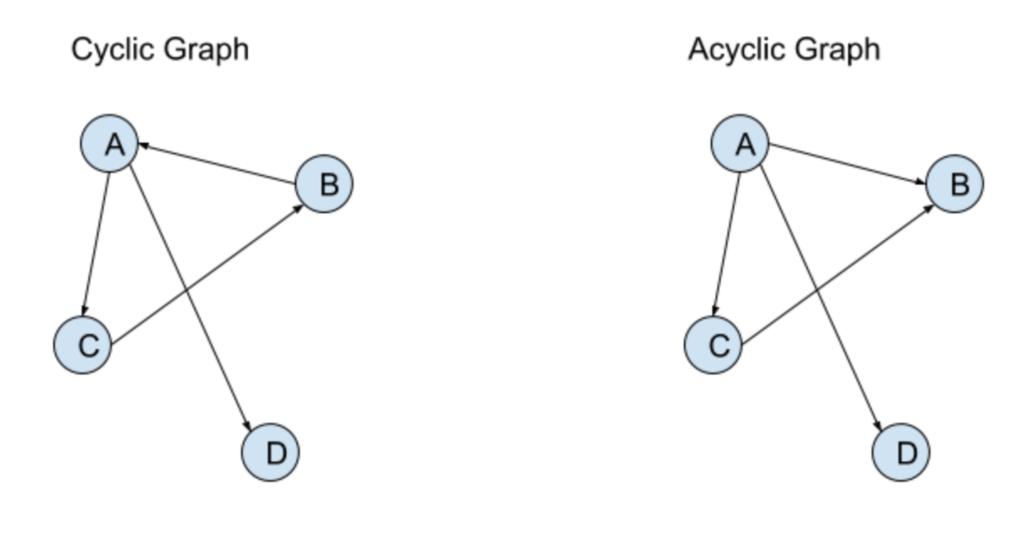
Acyclic vs Cyclic
If the graph has any pathway that can form a loop, then the graph is said to be cyclic [7]. On the other hand, an acyclic graph has no loops [7].
Typically, a user may decide to use directionality or weightiness depending on the application of the graph. Because of these various options available, graphs are useful to represent any network of objects that are interconnected in an intricate manner [4]. To understand how graph theory is used in computer science, let’s visit some common applications and algorithms.
Applications
Topological Sorting
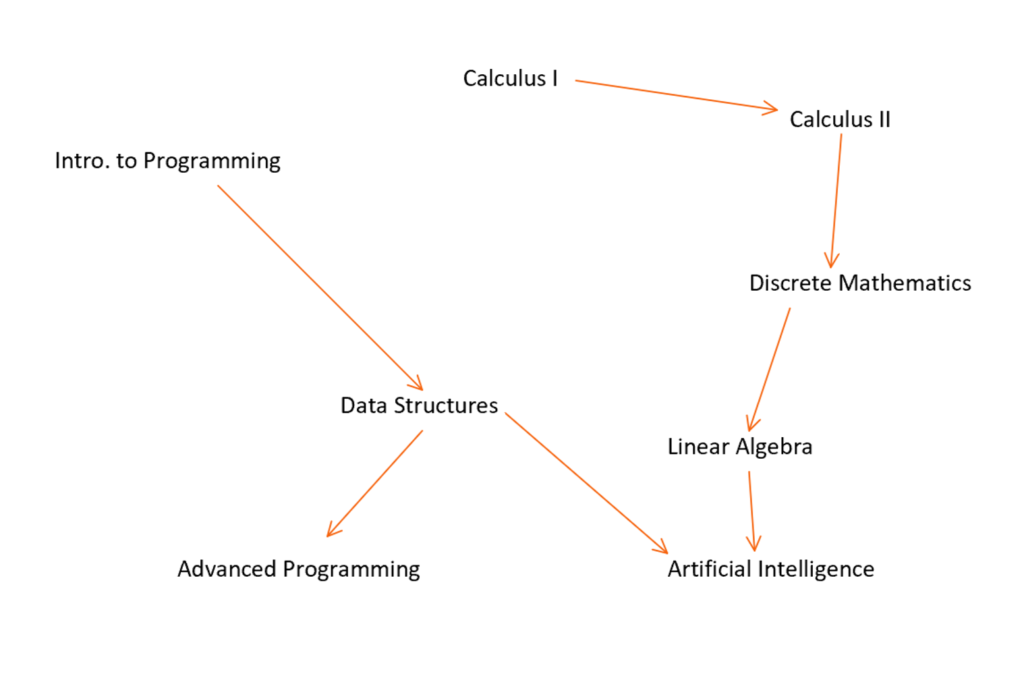
Suppose we have a directed acyclic graph, called DAG for short, there is at least one topological sorting possible [9]. In order to understand what topological sorting is, visit the figure below where which vertex represents a course, and the edge represents the pre-requisites of the course. For example, Calculus I is a pre-requisite for Calculus II. The topological sorting provides an ordered list of vertices in an order of which a student could take.
a
Figure 11 from flylib.com [10]
Firstly, we first must find the vertices that do not require any pre-requisites. To formalize this, this means that the vertex does not have any vertices directed to it. This character trait is termed as indegree. In figure 12, Introduction to Programming has an indegree of 0 and Linear Algebra has an indegree of 1. After visiting the first vertex A with an indegree of 0, in this case, Introduction to Programming, the algorithm must re-evaluate the indegrees for any course that has a pre-requisite of Introduction to Programming. This is done by visiting each adjacent vertex to A and decreasing the indegree by 1 [9]. Then, the algorithm repeats in a cycle, where it visits another vertex of an indegree of 0, such as Data Structures.
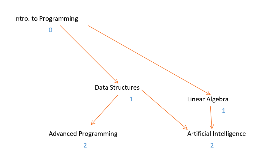
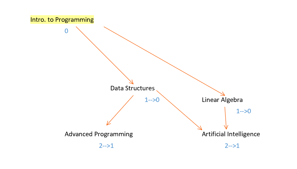
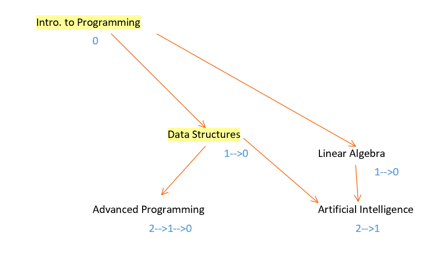
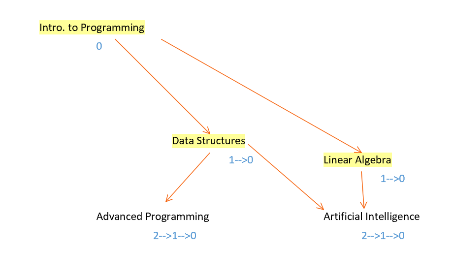
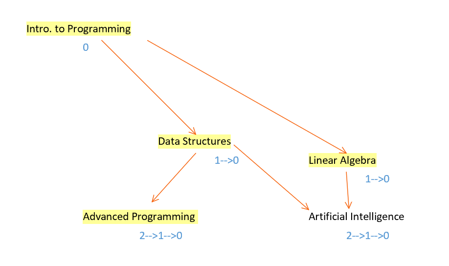
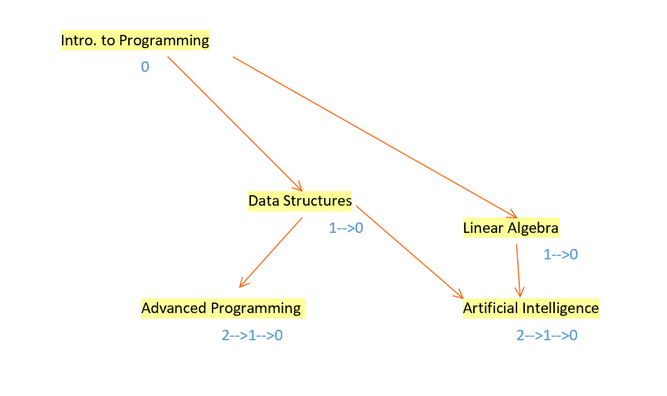
One of the possible pathways:
Intro. to Programming –> Data Structures –> Linear Algebra –> Advanced Programming
->Artificial Intelligence
Shortest Path
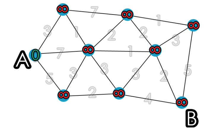
In an acyclic graph with non-negative edge weights, the shortest path from any given vertex to any other vertex can be determined [3]. This becomes helpful in graphically representations of maps and locations. If one were to have to run through several errands in New York City, what would be the most optimal? In a situation with 3-4 locations, the solution may be intuitive, but given any more locations such as 10, it can be difficult to deduce.
Dijkstra’s algorithm is a well-known greedy algorithm that finds the closest path from one given vertex [3], [11]. It accomplishes this by looking at its relative distance from the previously “found” vertices.
Each vertex is tied to additional parameters: distance (a decimal value), visited (boolean), and previous (vertex). The distance represents the relative distance from the starting vertex. The visited represents whether the vertex was already visited, and the previous allows the user to determine which vertex to visit before, for the shortest path. At the beginning of the algorithm, each vertex has a distance of infinity and a visited value of False [12].
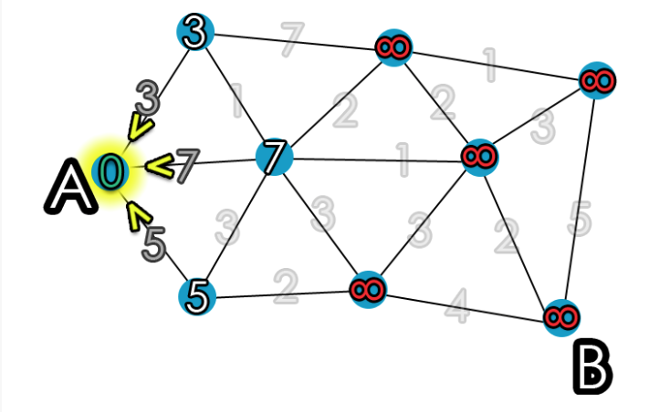
Suppose we are trying to figure out the shortest path from Vertex A, so the distance of Vertex A will be 0. Afterward, we will visit the vertex that has the smallest distance and one that has not been visited before. Now, vertex A’s visited variable is set to True, and the previous vertex would be none because it was the starting point.
Now the vertices adjacent to A will update its distance from A if it is smaller than the previous found distance.
Afterwards, the algorithm repeats until all vertices are visited by finding the next vertex with the smallest distance that has not been visited.
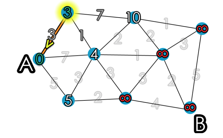
At the end of Dijkstra’s algorithm, the graph will formula the shortest path from A to every other vertex, ultimately forming a path from A to B as:
A –> 3 –> 4 –> 5 –> B
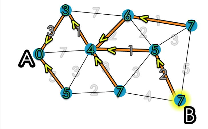
Dijkstra’s algorithm is a greedy algorithm because it solves the problem in stages by performing what is the best thing at each stage [12]. However, one limitation of Dijkstra’s algorithm is that it only finds the shortest path given a starting position. If Dijkstra’s algorithm was modified to find the shortest path from any starting point, then the cost would be severely larger because the operation would require a much longer runtime.
A famous problem, related to shortest paths, is a traveling salesman who wishes to visit several given cities and return to his starting point, in the shortest distance possible. However, this problem would be impossible to solve in a relatively cheap runtime because a lot of different combinations would have to be checked in the process [5], [12].
Centrality Problems
In graph analytics, centrality becomes an important concept when extracting key information from graphical networks [13]. In short, centrality determines how “central” a vertex is in a graph from other vertices [13].
Degree centrality is very similar to indegree, but it is used to determine relative importance of each vertex and can be used on undirected graphs [13]. To calculate the degree centrality, the number of edges connected to a vertex must be totaled.
Name: Degree Centrality:
Bob 3
Sally 2
Brenda 4
Ted 1
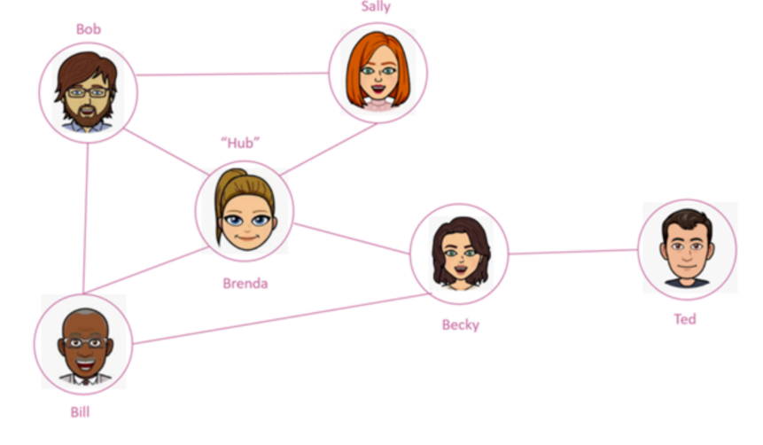
In this simple friend network, Brenda is the “Hub” which is important to users in the marketing industry [6], [13]. To simply put it, Brenda would have the ability to propagate any information to her social circle because she would have the most outreach. In a social network such as Twitter, the users with high degree centrality, such as celebrities, will have the most influence over the public, and this is why celebrities are paid to endorse products [13].
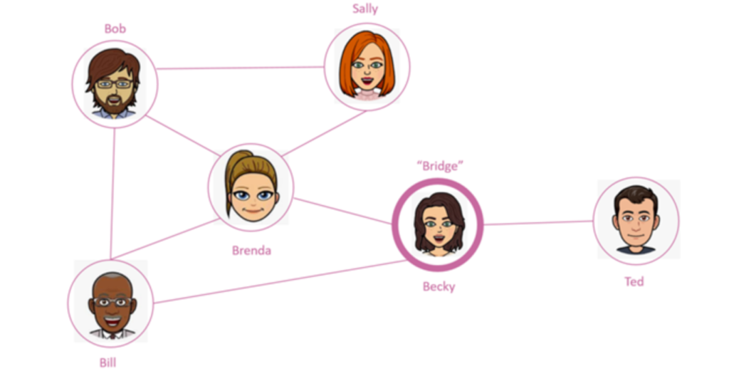
Betweenness Centrality measures how many times a vertex occurs in the shortest path between all pairs of vertices in a graph [6], [13]. The points with the high betweenness centrality are the “bridges” between different sets of vertices. In figure 23, it is evident that Becky is the sole link to Ted and the rest of the friends, hence she is the “bridge” [6], [13].
Similarly in figure 24, vertex A is the “bridge” connecting two different subgraphs together [13]. The importance of A can be thought of as, if A was removed from the graph, then there will be a major disconnect between the vertices in the graph [13].
There are several use cases of betweenness centrality such as determining different sub-graphs of a larger graph. For example, if the graph represented Facebook’s social network, then betweenness centrality can help determine different communities within Facebook’s larger social network [6], [13].
What else?
By no means, is this an exhaustive list or full exposure to Graph Theory, but it is the essentials. Graphs are among one of the most versatile models and can be used to display relations and connections in physical biology, and social systems [14]. Graphs allow for computer scientists to solve an endless amount of problems such as building a sudoku puzzle solver, determining efficient delivery routes, making a search engine, making two sub-graphs, determining clusters, etc [7]. Furthermore, we can anticipate more interplay with graph theory and new applications to come which will lead to even more ground-breaking developments.
Works Cited
[1] “The Real-Life Applications of Graph Data Structures You Must Know.” https://leapgraph.com/graph-data-structures-applications (accessed Nov. 23, 2020).
[2] “Graphs in Everyday Life – Graphs and Networks – Mathigon.” https://mathigon.org/course/graph-theory/applications (accessed Nov. 23, 2020).
[3] Ruohonen, Keijo, Graph Theory. 2013.
[4] “A Gentle Introduction To Graph Theory | by Vaidehi Joshi | basecs | Medium.” https://medium.com/basecs/a-gentle-introduction-to-graph-theory-77969829ead8 (accessed Nov. 24, 2020).
[5] R. J. Wilson, Introduction to graph theory, 4. ed., [Nachdr.]. Harlow: Prentice Hall, 20.
[6] “Using Facebook to learn some basics about graph theory | by Jessica Angier | Medium.” https://medium.com/@ja3606/using-facebook-to-learn-some-basics-about-graph-theory-ecadb31cd127 (accessed Nov. 24, 2020).
[7] “Don’t Understand Graphs? Here’s Why You Should Study Graphs in Computer Science | by Bennett Garner | Medium.” https://bennettgarner.medium.com/what-the-graph-a-beginners-simple-intro-to-graphs-in-computer-science-3808d542a0e5 (accessed Nov. 24, 2020).
[8] “Intro to Graphs – NY Comdori Computer Science Note.” https://nycomdorics.com/intro-to-graphs/ (accessed Nov. 24, 2020).
[9] “Topological Sort Tutorials & Notes | Algorithms | HackerEarth.” https://www.hackerearth.com/practice/algorithms/graphs/topological-sort/tutorial/ (accessed Nov. 24, 2020).
[10] “Topological Sorting | Graphs.” https://flylib.com/books/en/2.300.1/topological_sorting.html (accessed Nov. 24, 2020).
[11] “Dijkstra’s Shortest Path Algorithm | Brilliant Math & Science Wiki.” https://brilliant.org/wiki/dijkstras-short-path-finder/ (accessed Nov. 24, 2020).
[12] M. A. Weiss, Data structures and algorithm analysis in Java, 3rd ed. Upper Saddle River, N.J: Pearson, 2012.
[13] “Graph Analytics — Introduction and Concepts of Centrality | by Jatin Bhasin | Towards Data Science.” https://towardsdatascience.com/graph-analytics-introduction-and-concepts-of-centrality-8f5543b55de3 (accessed Nov. 24, 2020).
[14] R. PalSingh and V. Vandana, “Application of Graph Theory in Computer Science and Engineering,” IJCA, vol. 104, no. 1, pp. 10–13, Oct. 2014, doi: 10.5120/18165-9025.
[15] Images created by Shivani Patel.
[16] Featured Image provided by analyticsvidhya.com